Estimating solar X-ray flux

Once breakpoints can be detected and analyse, we can detect flares in real-time. However, detecting a flare does not imply that it is a strong flare, or that the electron density is high. Moreover, detecting a flare with one station does not mean that it will be detected with each station. Therefore, an additional layer is needed, which looks at all the results from the different stations, and synthetise them to publish an estimation of the solar X-ray flux and the flare importance.

The idea to do this is to use Bayesian statistics and the values of the phase variation compared to their quiet values (those variations are stored in the vlf4ions.class_definition.station.DP attribute, and computed by the compute_DA_DP() function).

Before using the code

Since the values of the phase variation may be dependent on different factors in addition to the solar X-ray flux, we cannot really link one value of DP to a single value of the Sun’s X-ray flux. Instead, we choose to measure DP for all flares on a time period (e.g. one year of data, similarly to the time period to compute the detection_threshold - see Breakpoints detection). From this, the various DP values can be discretized in bins, and the histograms detailing the flux probability can be computed for each DP bins, as seen below.

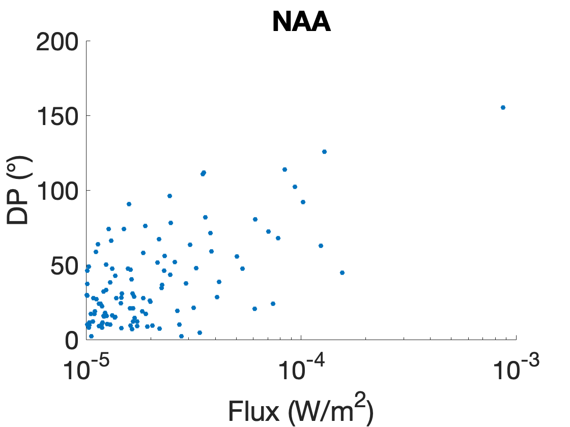
DP values for different flares with the NAA transmitter and the VLF receiver in Nançay

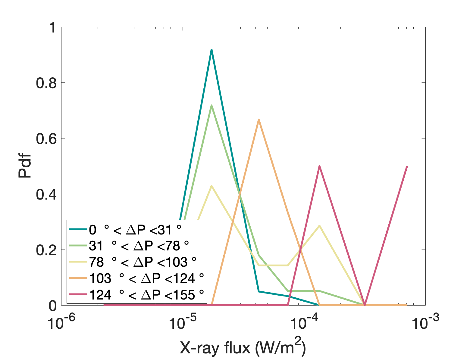
Probability density functions obtained from the previous graph, by discretising the different DP values.

Because the probability density functions seen just above may be too rough and too dependent on individual data points, we choose to fit them by gaussian distribution functions:

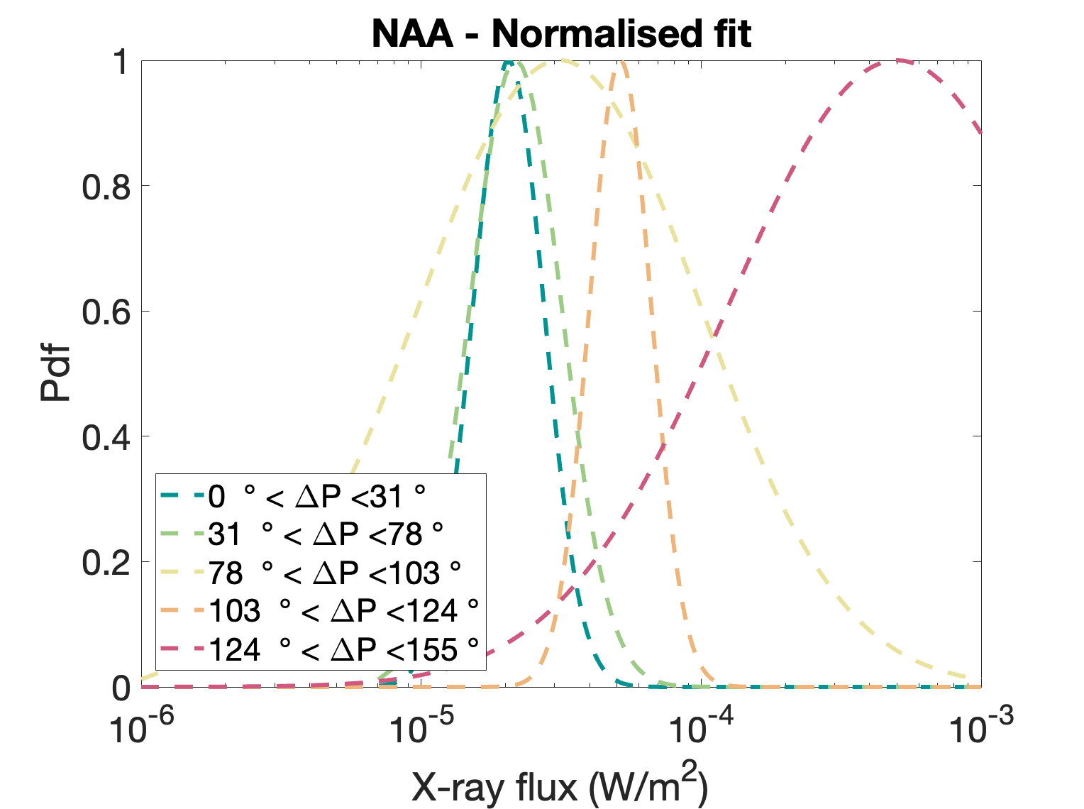
• The density function never goes to zero. This is crucial when combining probabilities since we do not want to completely exclude certain flux values. By ensuring the functions never go to zero, we let a small probability that the flux can be any value, and those probabilities may later increase depending on the values of DP for the other stations

• It means that we can store the values of the pdf as two numbers, mu and sigma. Those are attributes of the station class. They are stored in .csv files of the form seen below, where every line is another DP bin.

station_probas.csv

Low	High	mu	sigma
0	31	-5	1

Important

Thestation_probas.csv  files must have exactly this form. In the columnLow (resp.High) is stored the lowest (resp. highest) values of DP for each bin.muandsigma are the average and standard error of each gaussian probability density function for each DP bin. They are stored in units of log(flux) (i.e. a flux of 1e-4 W/m^2 for an X1 flare is-4).

Computation of DP

As described above, the main quantity for flux estimation is the DP value, which is the variation of the phase due to the solar flare. To compute this, we take the last quiet point (stored in the results files - see Results), for which we have kept both the detection time and the phase slope.

Using this, the phase that would have been measured had there been no solar flare can be estimated as

\[\phi_0 = \phi_{last_{quiet}} + p_1 * (time_{now} - time_{last_{quiet}})\]

DP can then be estimated as:

\[DP = \phi_{now} - \phi_0\]

Probability combination

Let’s suppose that we are following two transmitters, NAA and NSY. To obtain the complete solar flux estimation, we need to first have a first guess of the flux without any DP estimation and then to update this estimation each time we obtain a new estimation for DP for a station.

In practise, this is handled in the run() method.

From Bayes’ rule, we can write

\[P(flux|DP_{NAA}, DP_{NSY}, I) \propto P(flux| I) \times P(DP_{NAA}, DP_{NSY}|I)\]

where I represents any background information that we have. This gives:

\[P(flux|DP_{NAA}, DP_{NSY}, I) \propto P(flux| I) \times \frac{P(flux|DP_{NAA})}{P(flux|I)} \times \frac{P(flux|DP_{NSY})}{P(flux|I)}\]

if we assume that the values of \(DP_{NSY}\) and \(DP_{NAA}\) are independent. This can be generalised to any number of transmitters.

Prior

In the above equations, we call \(P(flux|I)\) as the prior. This is in fact the probability of the flux being a certain value, given that there was a detection. Since detections can occur for any type of solar flare, this is taken as a uniform prior from 1e-6 to 1e-3 W/m^2.

Note

While the prior is uniform, it is not the case of the probability flux distribution when DP` is 0. Indeed DP = 0 gives us important information: it implies that for a specific station, we are in quiet times. Therefore, in this cas, the probability distrubution function that is returned is a gaussian centered in C1 and with a sigma of 1 (log(W/m^2^)).

Results

Results in post-processing:

This method was employed on three flares detected with NAA, NRK and NSY with the AWESOME instrument in Nançay. It should be noted that none of the flares were used to build the probability density functions used for the flux estimation.

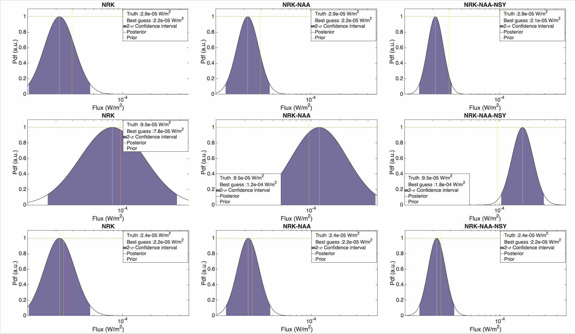
Flux estimation for three flares occuring in November and December 2024.

All flux were estimated within a factor of 2. It should be noted that using more station doesn’t necessarily improve the flux estimation; however, it lowers its uncertainty and limits the number of false detections. It also ensures that flares can be detected even in case of transmitter failure.

Results in real-time:

In real-time, we do not have access to GOES flux data. What is returned are probability distribution functions when the run() method is called, not at the peak of the flare. Each time this method is called, it generates two graphs (see Results). The one of interest here is calledlast.pdfand presents the probability distribution function computed with the available stations (which are transmitting and not in nighttime). Below is an example of posterior distribution function

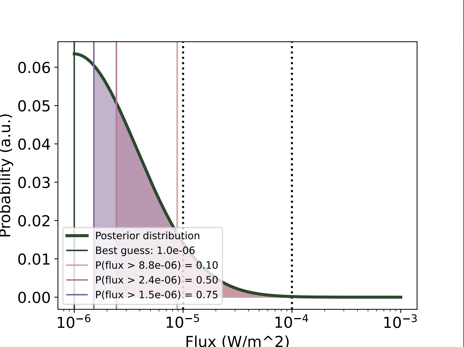
Probability distribution function returned in quiet time

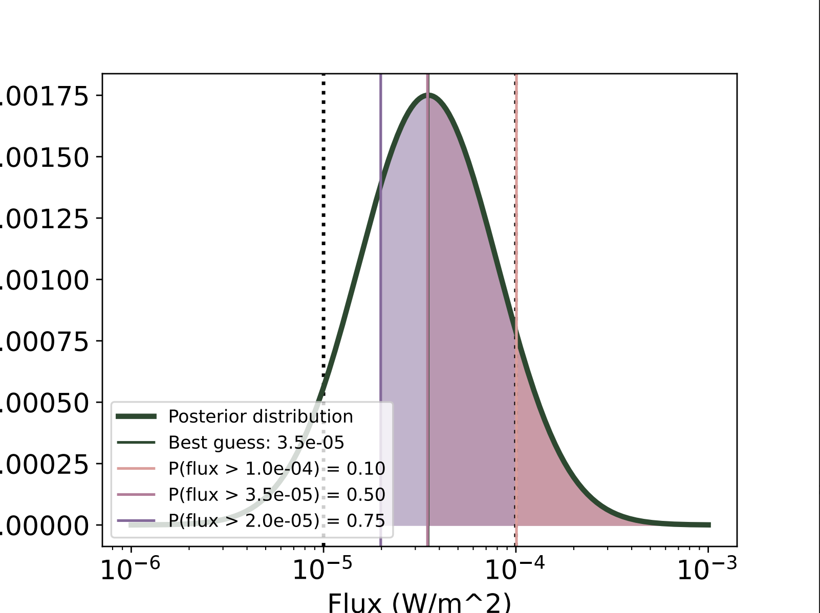
Probability distribution function returned for a flare

Note

In each case, the posterior distribution function is returned along with associated thresholds (the probability of the flux being above those thresholds is 0.1, 0.5 or 0.75). As visible in the first figure, the posterior distribution function in quiet times is ‘cut’, and the thresholds are not correct. This could be corrected, but it is not a priority right now.

Thresholds can be used to generate alerts (see Alerts).

Each time the nowcast.run() method is called, a result file is also created, containings the best estimate for the flux, the number of stations transmitting in daytime at the time, and a measure of whether it is a quiet or flare time. This last parameter is indicated by a number between 0 and 1, proportional to the number of working station which are in quiet times. If this number is 1, all stations are in quiet time. If it is 0, all stations have detected a flare.